In one of the recent posts by T. Tao on the progress of the Polymath8 project, the question arose of whether such functions as
$latex \varphi(x)=\sum_{y\in\mathbf{F}_p} e\Bigl(\frac{f(x,y)}{p}\Bigr)$
defined for $latex x\in\mathbf{F}_p$ and a rational function $latex f\in\mathbf{F}_p(X,Y)$, are trace functions, and more importantly, what is their conductor (see this, and the following, comments). In particular, if $latex f$ is obtained by reduction modulo primes of a fixed rational function in $latex \mathbf{Q}(X,Y)$, one could expect that the answer is “Yes”, with a bound for the conductor independent of $latex p$.

This is in fact a question that É. Fouvry, Ph. Michel and I had considered in special cases (or variants) in some of our papers. In fact, it is natural to consider more generally the linear map sending a function $latex K\,:\, \mathbf{F}_p\rightarrow \mathbf{C}$ to the function
$latex \varphi(x)= T_{f}(K)(x)=\sum_{y\in\mathbf{F}_p} K(y) e\Bigl(\frac{f(x,y)}{p}\Bigr),$
(which is an analogue of an integral operator) and to ask whether this linear map sends trace functions to trace functions, and if yes, if the conductor of $latex \varphi$ is bounded in terms of the conductor of $latex K$ and the degree of the numerator and denominator of $latex f$.

The most important case, which is crucial in all our series of papers, is the Fourier transform, which corresponds simply to $latex f(X,Y)=XY$. We proved the desired property (which we view, rather naturally I think, as a form of “continuity” of the Fourier transform, in an algebraic sense) in that case using Deligne’s definition and Laumon’s study of the sheaf-theoretic Fourier transform. Most importantly, in order to estimate the conductor of the Fourier transform of a trace function, we used Laumon’s theory of the local Fourier transform, which is rather deep.

It is by no means clear (and this is a rather interesting question of algebraic geometry!) that such a local theory exists, and leads to the continuity property, for arbitrary “kernels” $latex e(f(x,y)/p)$. However, we figured out a way to prove the conductor bound that bypasses these local results. It applies to the Fourier transform, and although it is then much less precise than what is obtained from Laumon’s theory, it gives a (possibly) more accessible proof of the continuity property.

We have just put here our preprint with this result. It is not yet submitted to arXiv because we are considering various possibilities for either extensions of applications, but the proof of the main result is complete.

The paper was rather interesting to write. On the one hand, it turns out that it is not needed for the original question from Polymath8: Philippe found an elementary argument that reduces the specific example of the problem which reduces it, essentially, to a special case of the Fourier transform (this is written down in the Deligne section of the Polymath8 paper). On the other hand, although we had thought a bit about this question beyond the Fourier transform, we had not made progress. The reason, in retrospect, is that in order to treat the general transform
$latex T_{f}(K)(x)$
(as defined above), we begin by treating the special case
$latex T_f(1)(x)=\sum_{y\in\mathbf{F}_p} e\Bigl(\frac{f(x,y)}{p}\Bigr),$
and without the motivation from the Polymath8 project, we had not thought of this first step.

The reason that things work this way is, as all other main ideas in this paper, very easy to explain by writing down and manipulating sums, and assuming that those behave always as the best Riemann Hypothesis over finite fields suggest. But the actual arguments are purely algebraico-geometric, and we end up using quite a bit of the general formalism of étale cohomology, but not the Riemann Hypothesis (which is morally as things should be.)

I will give here the informal sketch: first of all, the function
$latex \varphi(x)= T_{f}(K)(x)=\sum_{y\in\mathbf{F}_p} K(y) e\Bigl(\frac{f(x,y)}{p}\Bigr),$
is indeed a trace function if $latex K$ is one, in almost all cases: precisely, the existence of higher-direct image sheaves with compact support, the proper base change theorem, and the Grothendieck trace formula, show that
$latex \varphi(x)=t_0(x)-t_1(x)+t_2(x),$
where $latex t_i$ is the trace function of the sheaf
$latex R^ip_{1,!} (p_2^*\mathcal{F}\otimes \mathcal{L}),$
where $latex p_1,\ p_2$ are the two projections $latex (x,y)\mapsto x$ and $latex (x,y)\mapsto y$, the sheaf $latex \mathcal{F}$ is the one with trace function $latex K$, and the sheaf $latex \mathcal{L}$ is the Artin-Schreier sheaf on the plane with trace function
$latex t_{\mathcal{L}}(x)=e(f(x,y)/p)$
for $latex x,\ y\in\mathbf{F}_p$. In many cases, both $latex t_0$ and $latex t_2$ vanish, and then $latex \varphi$ is (minus) the trace function of the sheaf
$latex \mathcal{G}=R^1p_{1,!} (p_2^*\mathcal{F}\otimes \mathcal{L}).$

This essentially answers the first question in full generality: the “transform” $latex K\mapsto T_f(K)$ maps trace functions to trace functions.

Now consider the conductor of the sheaf $latex \mathcal{G}$ above. We defined it as the sum of three terms. Two are relatively accessible: they are the (generic) rank of the sheaf, and the number of singularities. We can basically determine these if we know the dimension of all fibers: the maximum dimension gives an upper bound for the rank, and a result of Deligne says (roughly) that the singularities are the points where the fiber has smaller than maximal dimension. So let us assume that we can bound these quantities for the transform sheaf $latex \mathcal{G}$. Then there only remains to estimate the third term, which is the sum of the Swan conductors at the singularities. This is rather delicate, at least for people for whom — and this applies to us… — the Swan conductor remains a rather mysterious and subtle data.

The first idea is that, assuming the other two pieces of the conductor are under control, the sum of the Swan conductors is bounded by a global invariant that may be accessible in applications. Namely, if a sheaf $latex \mathcal{M}$ is lisse on a dense open subset $latex U$ of the affine line then the Euler-Poincaré characteristic formula (of Néron, Ogg, Shafarevitch) easily proves that
$latex \sum_x \mathrm{swan}_x(\mathcal{M})\ll \text{(rank of }\mathcal{M}\text{)}+ \text{(nb. of sing.)} + \dim H^1_c(\bar{U},\mathcal{M}).$
So we have to deal with the dimension of the cohomology group $latex H^1_c(\bar{U},\mathcal{M})$. The point is that, in good circumstances, and especially if $latex \mathcal{M}$ is of weight $latex 0$, we can expect that
$latex \dim H^1_c(\bar{U},\mathcal{M})=\limsup p^{-n/2} |S_n|,$
where $latex S_n$ is the sum of the trace function of $latex \mathcal{M}$ over the points of $latex U(\mathbf{F}_{p^n})$. Estimating this becomes a problem of analytic number theory, and we may hope to succeed.

For instance, if we apply this principle to
$latex \mathcal{M}=R^1p_{1,!}\mathcal{L},$
with $latex \mathcal{L}$ the Artin-Schreier sheaf associated to a rational function $latex f$ as before, the sum $latex S_n$ is simply
$latex p^{-n/2}S_n=\frac{1}{p^{n/2}}\sum_{x\in U(\mathbf{F}_{p^n})}\sum_{y\in\mathcal{F}_{p^n}}e\Bigl(\frac{\mathrm{Tr}_nf(x,y)}{p}\Bigr),$
were $latex \mathrm{Tr}_n$ is the trace from $latex \mathbf{F}_{p^n}$ to $latex \mathbf{F}_p$.

In good circumstances, we know square-root cancellation for this two-variable character sum, and we obtain a bound for the limsup of $latex p^{-n/2}S_n$, which depends only on the degree of the numerator and denominator of $latex f$, using Bombieri’s bounds for sums of Betti numbers for such exponential sums (or the generalizations of Adolphson-Sperber, or those of Katz.)

This deals (optimistically) with the transform with kernel $latex \mathcal{L}$ when the input sheaf is the trivial sheaf, which we note is the case in the Polymath8 case. Now for the second idea: assume we consider
$latex \mathcal{M}=R^1p_{1,!}(_2^*\mathcal{F}\otimes\mathcal{L})$
now, and try to use the same principle. With $latex K$ denoting the trace function of $latex \mathcal{F}$, the sum $latex S_n$ now satisfies
$latex p^{-n/2}S_n=\frac{1}{p^{n/2}}\sum_{x\in U(\mathbf{F}_{p^n})}\sum_{y\in \mathbf{F}_{p^n}} K(y)e\Bigl(\frac{\mathrm{Tr}_nf(x,y)}{p}\Bigr).$

In impeccable style, we exchange the two sums of course. We get
$latex p^{-n/2}S_n=\frac{1}{p^{n/2}}\sum_{y\in \mathbf{F}_{p^n}} K(y) \sum_{x\in U(\mathbf{F}_{p^n})}e\Bigl(\frac{\mathrm{Tr}_nf(x,y)}{p}\Bigr)=\frac{1}{p^{n/2}}\sum_{y\in \mathbf{F}_{p^n}} K(y)L(y)$
where
$latex L(y)=\sum_{x\in U(\mathbf{F}_{p^n})}e\Bigl(\frac{\mathrm{Tr}_nf(x,y)}{p}\Bigr).$
But, by the first step, applied to $latex f^*(X,Y)=f(Y,X)$ instead of $latex f(X,Y)$, the function $latex L$ is a trace function with conductor bounded in terms of the degrees of $latex f^*$, or equivalently of $latex f$. Thus $latex p^{-n/2}S_n$ is the inner-product, over $latex \mathbf{F}_{p^n}$, of the trace functions of two sheaves with bounded conductor, and we can expect both to have weight $latex 0$. We can then expect quasi-orthogonality from the Riemann Hypothesis, and a resulting bound for the limsup that depends only on the conductors of these two sheaves, i.e., on the conductor of $latex \mathcal{F}$ (for $latex K$) and on the degrees of the numerator of denominator of $latex f$ (for $latex L$). This is the desired conclusion.

This sketch explains why we can prove the results in our paper. In many cases, it is certainly a valid reasoning, but it is not easy to make it rigorous in great generality. The basic problems are that it depends on the sums $latex S_n$ having square-root cancellation (which for the transform of the trivial sheaf is a non-trivial assumption), and also on $latex S_n$ detecting all of the cohomology space, and not just the part of weight $latex 1$: by Deligne’s Riemann Hypothesis, the eigenvalues of Frobenius on $latex H^1_c(\bar{U},\mathcal{G})$ are of weight $latex \leq 1$ if $latex \mathcal{G}$ has weight $latex 0$, but the limsup only gives the number of eigenvalues of weight $latex 1$, and having too many smaller eigenvalues would create problem.

We work around these possible difficulties by dropping the diophantine motivation, and going straight at the dimension of $latex H^1_c(\bar{U},\mathcal{G})$. To do this, we need algebraic analogues of the two fundamental analytic steps we used:

(1) expressing the sum $latex S_n$ for the trivial sheaf as a two-variable character sum;

(2) exchanging the order of the two sums when inserting a general input sheaf $latex \mathcal{F}$.

Both of these are replaced by (very elementary) arguments with Leray spectral sequences. This is a relatively well-known idea (it is part of the “dictionary” in Deligne’s survey on Sommes trigonométriques in SGA 4 ½ and quite a few concrete examples are found in papers and books of Katz), but it is the first time we use it ourselves. I will survey and explain this in a later post, since it seems that a good concrete example of the use of spectral sequences in analytic number theory might be a useful thing to have somewhere…

The reader who opens the PDF file of our preprint might be surprised to see that the paper in more than thirty pages long, in comparison with the rather simple-looking discussion above. The length is justified partly by the two motivating discussions we have included (the diophantine argument with $latex S_n$, and a self-contained algebraic treatment of the important case of the Fourier transform). But it also turns out that taking care of the “easy” parts of the conductor requires somewhat lengthy elementary arguments with rational functions. Most importantly maybe, we must take into account the fact that, in contrast with our previous works, we now have to handle general constructible $latex \ell$-adic sheaves, and not only middle-extension sheaves: there is no reason for our transformed sheaves to be so-well behaved in general. This requires adding a further component to the conductor (roughly, the support and dimension of the fibers of the “punctual part” of the sheaf, e.g., the conductor of a sheaf supported at $latex 0$ with fiber of dimension $latex n\geq 1$ must increase with $latex n$), and we also need to control it before applying the previous ideas. We also prove, both as a useful too and as a by-product, the analogue of the Bombieri bounds for a general input sheaf $latex \mathcal{F}$: the Betti numbers
$latex \dim H^i_c(\mathbf{A}^2\times\bar{\mathbf{F}}_p,p_2^*\mathcal{F}\otimes \mathcal{L})$
are bounded in terms of the conductor of $latex \mathcal{F}$ and the degree of the numerator and denominator of $latex f$.

In my series of papers with É. Fouvry and Ph. Michel, we seem to alternate between longer papers and shorter ones. The last one, which we just put up on arXiv, is in some sense the shortest one: even if it goes up to 19 pages in length, the basic idea can be explained extremely quickly, and much of the paper is taken with variations on its basic theme and illustrations.

The context is the all-important problem of estimating short exponential sums, in the specific case of sums over intervals in a cyclic group $latex A=\mathbf{Z}/m\mathbf{Z}$, where (for the sake of this post) we define an interval $latex I$ in $latex A$ to be the injective image of a set of successive integers under reduction modulo $latex m$. An interval is “short” if its length is significantly smaller than $latex m$, in the sense that $latex |I|=m^{\theta}$ for some real parameter with $latex 0\leq \theta<1$. We are then looking for non-trivial estimates for
$latex \sum_{x\in I}\varphi(x)$
where $latex \varphi\,:\, A\rightarrow \mathbf{C}$
is some complex-valued function, which is supposed to oscillate in such a way that we expect that
$latex \sum_{x\in I}\varphi(x)=o(|I|\|\varphi\|_{\infty}).$

There is a fundamental technique to attack this problem, which is of constant use in analytic number theory, and which is known as the completion method. Abstractly, one can see it as a case of the Plancherel formula in (discrete) Fourier analysis, namely, one writes
$latex \sum_{x\in I}\varphi(x)=\sum_{t\in A}\hat{\varphi}(t)\hat{I}(t),$
where
$latex \hat{\varphi}(t)=\frac{1}{\sqrt{m}}\sum_{x\in A}\varphi(x)e\Bigl(\frac{tx}{m}\Bigr),$
and $latex \hat{I}$ is the same transform applied to the characteristic function of the interval $latex I$. One then deduces the bound
$latex \sum_{x\in I}\varphi(x)\ll \|\hat{\varphi}\|_{\infty}\sqrt{m}(\log m),$
where the implied constant is absolute, simply by estimating the $latex L^1$-norm of $latex \hat{I}$ — in our normalization, this is $latex \ll \sqrt{m}(\log m)$.

In many cases, the Fourier transform of $latex \varphi$ can be estimated quite well, and in particular, in the context of finite fields $latex A=\mathbf{F}_p$, if $latex \varphi$ is a trace function which is not proportional to an additive character $latex e(x/p)$, Deligne’s Riemann Hypothesis gives
$latex \|\hat{\varphi}\|_{\infty}\ll 1,$
where the implied constant depends only on the conductor of (the sheaf underlying) $latex \varphi$.

The resulting estimate
$latex \sum_{x\in I}\varphi(x)\ll \sqrt{m}(\log m)$
is known as the general Polya-Vinogradov bound (although the name is sometimes restricted to the case where $latex \varphi=\chi$ is a Dirichlet character modulo $latex m$.)

This is quite an efficient result: it gives non-trivial estimates for all intervals $latex I$ such that $latex p/(\log p)=o(|I|)$ (or even $latex |I|=c\sqrt{p}(\log p)$, for a suitable $latex c>0$, if one only desires some cancellation by a multiplicative constant, and not that the sum be of smaller order of magnitude.) With this generality, it is also almost best possible: if we take $latex \varphi(x)=e(x^2/p)$, then the sum over $latex 1\leq x\leq \sqrt{p}$ has essentially no cancellation (the phase does not have enough time to turn around sufficiently.)

It seems natural, then, to ask: is the Polya-Vinogradov range (where $latex I$ is a bit larger than $latex \sqrt{p}(\log p)$) best possible? Does the gap between $latex \sqrt{p}$ and $latex \sqrt{p}(\log p)$ really represent a different behavior for such generalized exponential sums?

Our paper answers this question quite satisfactorily: there is, in fact, no gap, in the sense that for trace functions (not proportional to an additive character), one can get cancellation in sums over intervals of length $latex \sqrt{p}\beta(p)$ for any function $latex \beta(p)$ tending to infinity with $latex p$ (assuming we do tend to infinity while keeping the conductor bounded.)

As a direct corollary, we get for instance the equidistribution in $latex [0,1]$ (with respect to Lebesgue measure) of fractional parts $latex \{\frac{f(n)}{p}\}$ for $latex 1\leq n\leq \sqrt{p}\beta(p)$, for any fixed polynomial $latex f\in \mathbf{Z}[X]$ of degree $latex \geq 2$, and the equidistribution with respect to the Sato-Tate measure of the angles of Kloosterman sums $latex \theta_p(x)$ such that
$latex \frac{1}{\sqrt{p}}\sum_{y\in\mathbf{F}_p^{\times}}e\Bigl(\frac{xy+y^{-1}}{p}\Bigr)=2\cos\theta_p(x),$
again for $latex 1\leq x\leq \sqrt{p}\beta(p)$, whenever $latex \beta(p)\rightarrow +\infty$. (This last result had been proved in the Polya-Vinogradov regime by Philippe a while ago, and in the full range $latex 1\leq x\leq p-1$, it is a celebrated result of Katz.)

As I mentioned, the basic method is very easy, and we call it the “sliding sum method”. It is reminiscent of the van der Corput inequality, and we wouldn’t be surprised to learn that it had already been established by other people. (The applicability to trace functions, on the other hand, requires some rather deep results, as I will discuss below.)

I will give the simplest variant. Consider an interval $latex I$ in $latex A=\mathbf{Z}/m\mathbf{Z}$. We assume that $latex |I|=\sqrt{m}\beta$ with $latex \beta=\beta(I)\geq 1$ (so we are certainly above the square-root length). We then compare upper and lower bounds for the average
$latex \Sigma=\sum_{a\in A}{\Bigl|\sum_{x\in I}{\varphi(x+a)}\Bigr|^2}.$

For the upper-bound, we expand the square and exchange the order of summation, obtaining
$latex \Sigma=\sum_{x,y\in I}C(\varphi;x-y)$
where
$latex C(\varphi,t)=\sum_{a\in A}\varphi(a)\overline{\varphi(a+t)}$
is an additive correlation sum of $latex \varphi$ (it is a special case of those correlation sums we have considered extensively in our first works.)

We assume that $latex \varphi$ has the property that, if $latex t$ is not in a set containing at most $latex c$ values, we have
$latex |C(\varphi,t)|\leq c \sqrt{m}$
(i.e., the correlation exhibits uniform square-root cancellation, except for a few exceptional cases, among which of course we expect to have $latex t=0$). Then, using the trivial bound
$latex |C(\varphi,t)|\leq \|\varphi\|_{\infty}^2m$
for the exceptional values of $latex t=x-y$, we get
$latex \Sigma\ll m|I|+m^{1/2}|I|^2\ll m^{1/2}|I|^{1/2},$
where the implied constant depends on the parameter $latex c$ that we just introduced, and on the $latex L^{\infty}$-norm of $latex \varphi$ (and we use the fact that $latex |I|\geq \sqrt{m}$.)

As for the lower bound, we just use the fact that if we shift $latex I$ by a small amount, the sum over $latex a+I$ does not change too much (because the interval and its shift overlap significantly; intuitively, we slide the sum over a certain range, hence our name for the method):
$latex \Bigl|\sum_{x\in I}\varphi(x)-\sum_{x\in I}\varphi(x+a)\Bigr|\leq 2|a|\|\varphi\|_{\infty}.$

This means that if we consider the sums shifted by $latex a$ of size up to (roughly) the sum
$latex S=\sum_{x\in I}\varphi(x)$
itself, these will have a contribution to $latex \Sigma$ of size roughly $latex \gg |S|^3.$ So by comparing the upper and lower bounds (using positivity), we get
$latex |S|^3\ll m^{1/2}|I|^2,$
or, in terms of the parameter $latex \beta\geq 1$, we get
$latex S\ll |I|^{2/3}m^{1/6}=|I|\beta^{-1/3}$
(where the implied constant depends on $latex c$ and on $latex \|\varphi\|_{\infty}$).

Hence, provided we work with functions with bounded $latex L^{\infty}$-norm and with uniformly small correlations in the sense we described, then we can get cancellation as long as $latex \beta(I)\rightarrow +\infty$, but arbitrarily slowly.

This is elementary, but now the really significant part is that if $latex \varphi$ is a trace function modulo $latex m=p$, and if it is associated to an irreducible sheaf, and is not proportional to an additive character, then it does have the desired properties, the parameter $latex c$ being bounded in terms of the conductor $latex c(\varphi)$ of $latex \varphi$ (which also satisfies $latex \|\varphi\|_{\infty}\leq c(\varphi)$, so that it serves as a universal complexity parameter, as it did in our previous works.)

We do not need to fight very hard to prove this in our new paper, but this is because we can quote and use various lemmas from the previous ones, and — as usual — rely on Deligne’s fundamental version of the Riemann Hypothesis over finite fields; the result itself is undoubtedly quite deep when applied to trace functions which are not of rank $latex 1$.

As a last remark: the method is robust, and we adapt it for instance to sums over proper generalized arithmetic progressions, which are natural generalizations of intervals. Here we get bounds of quality depending also on the dimension of the progression (the saving $latex \beta^{-1/3}$ is replaced by $latex \beta^{-1/(k+2)}$ for a $latex k$-dimensional progression), but the result is appealing even for large $latex k$ because the Polya-Vinogradov gap is
$latex \sqrt{m}\leq |B|\leq \sqrt{m}(\log m)^k$
for a $latex k$-dimensional progression $latex B\subset \mathbf{Z}/m\mathbf{Z}$, hence its size also increases with $latex k$ (this follows from a recent result of X. Shao bounding the $latex L^1$-norm of the Fourier transform of the characteristic function of $latex B$.)

I more or less designated myself as the official photographer of the Fouvry60 conference, and took many pictures, quite a few of which turned out rather well. Certainly, when I view them, I think they give an accurate impression of the atmosphere of the conference. In this post I will just preview a very small selection — I and the other organizers are attempting to find the best way to make the full set available for the participants (at least.)

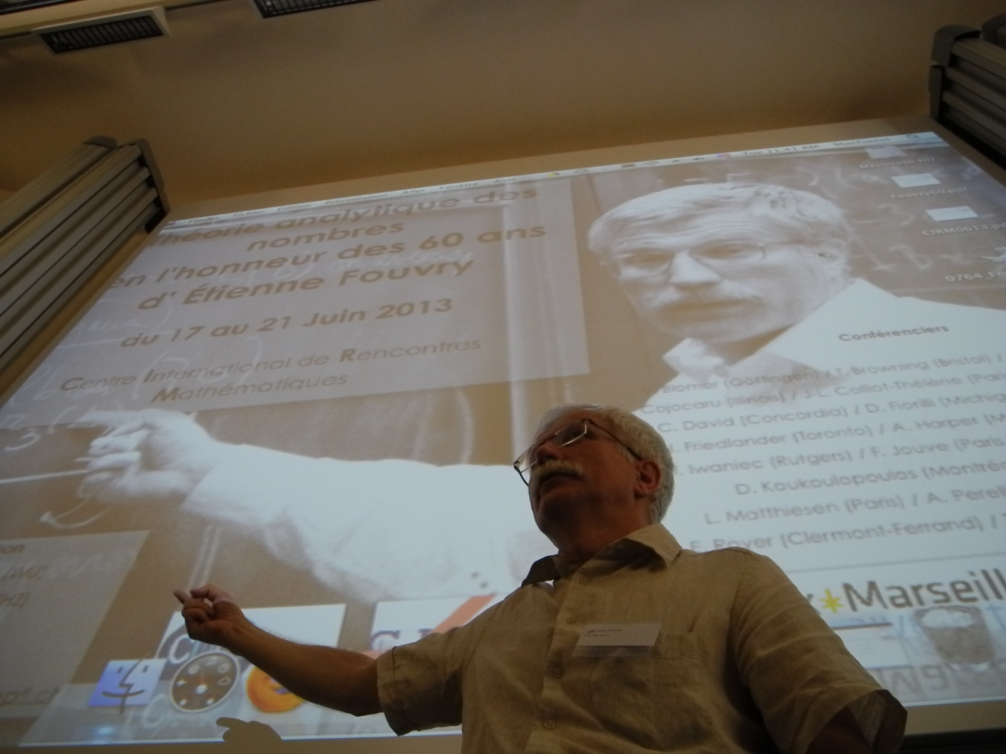
Although Jean-Marc Deshouillers could only attend the first day of the meeting, I was very happy to be able to take a good picture to remind us all of Kloostermania…

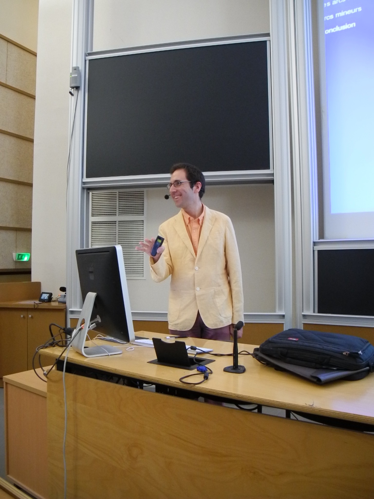
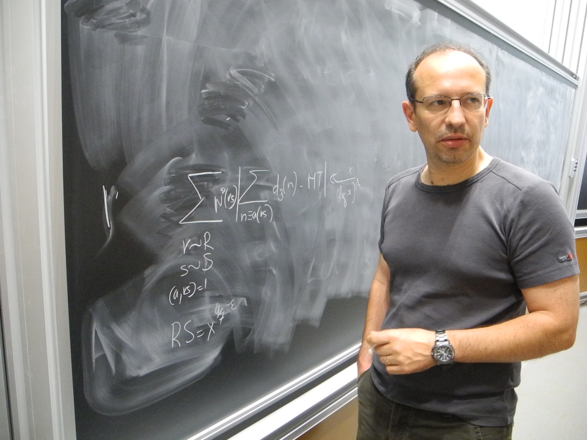
Voted best-dressed speaker, and speaking about the ternary Goldbach problem, here is Harald Helfgott.

The picture for the poster was taken by C.J. Mozzochi around 1999 in Princeton.

Any time we use Pari/GP for number-theoretic computations, we can thank Karim and Henri (and a few others) for their work; Henri is currently working on a new modular forms script for Pari…

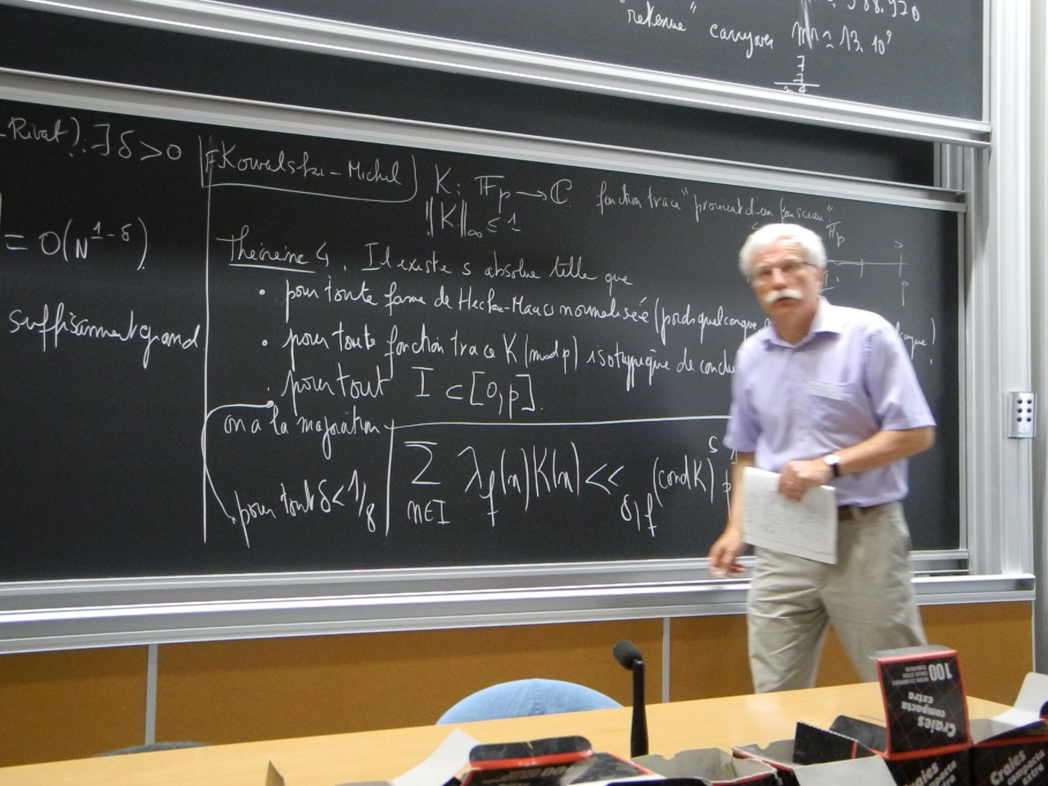
Henryk Iwaniec presented his work with Brian Conrey in extending the Levinson-Conrey method to allow long mollifiers.

Cécile Dartyge, before she presented her very impressive work on the largest prime divisors of values of a polynomial of degree $latex 4$.

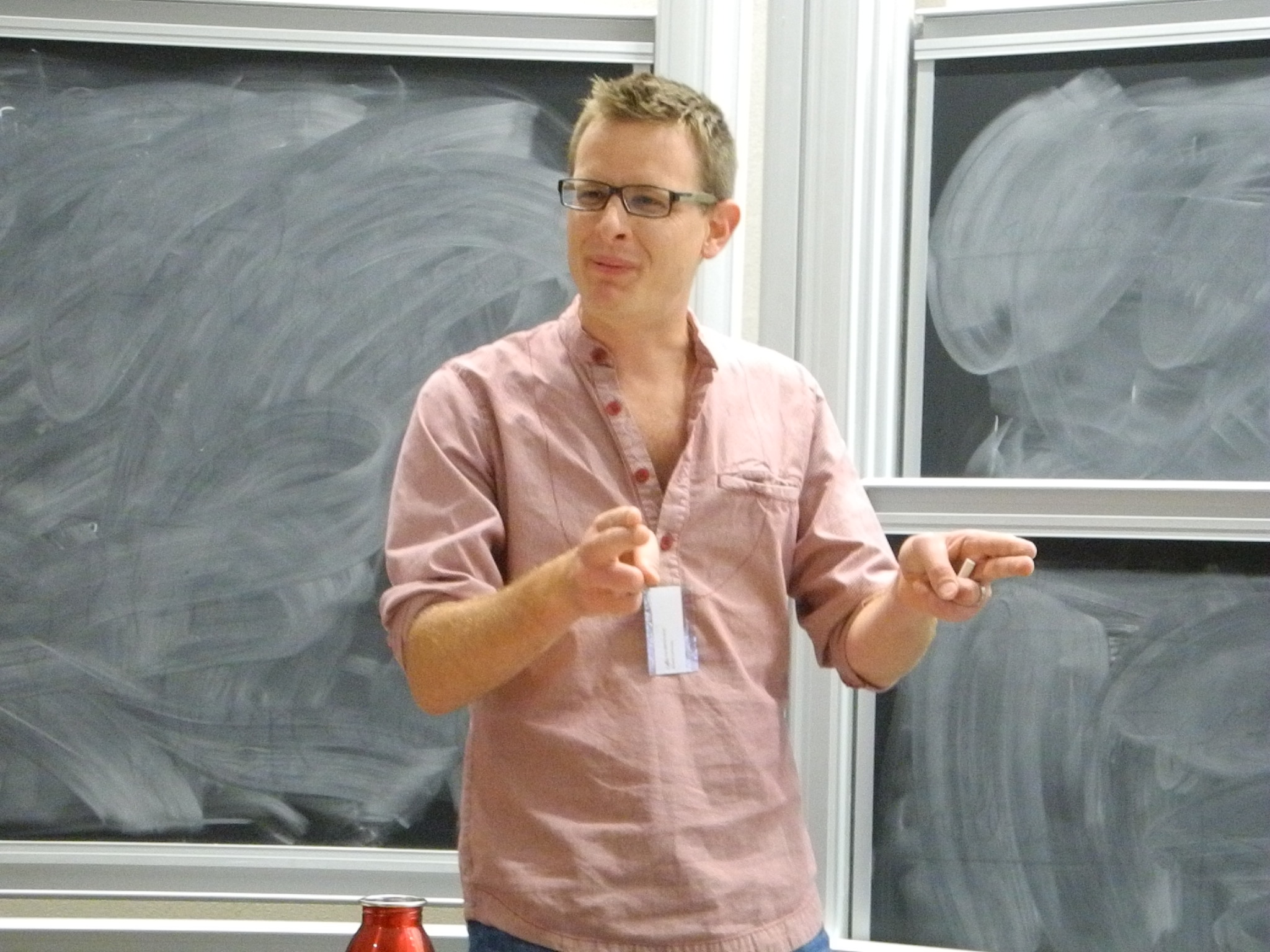
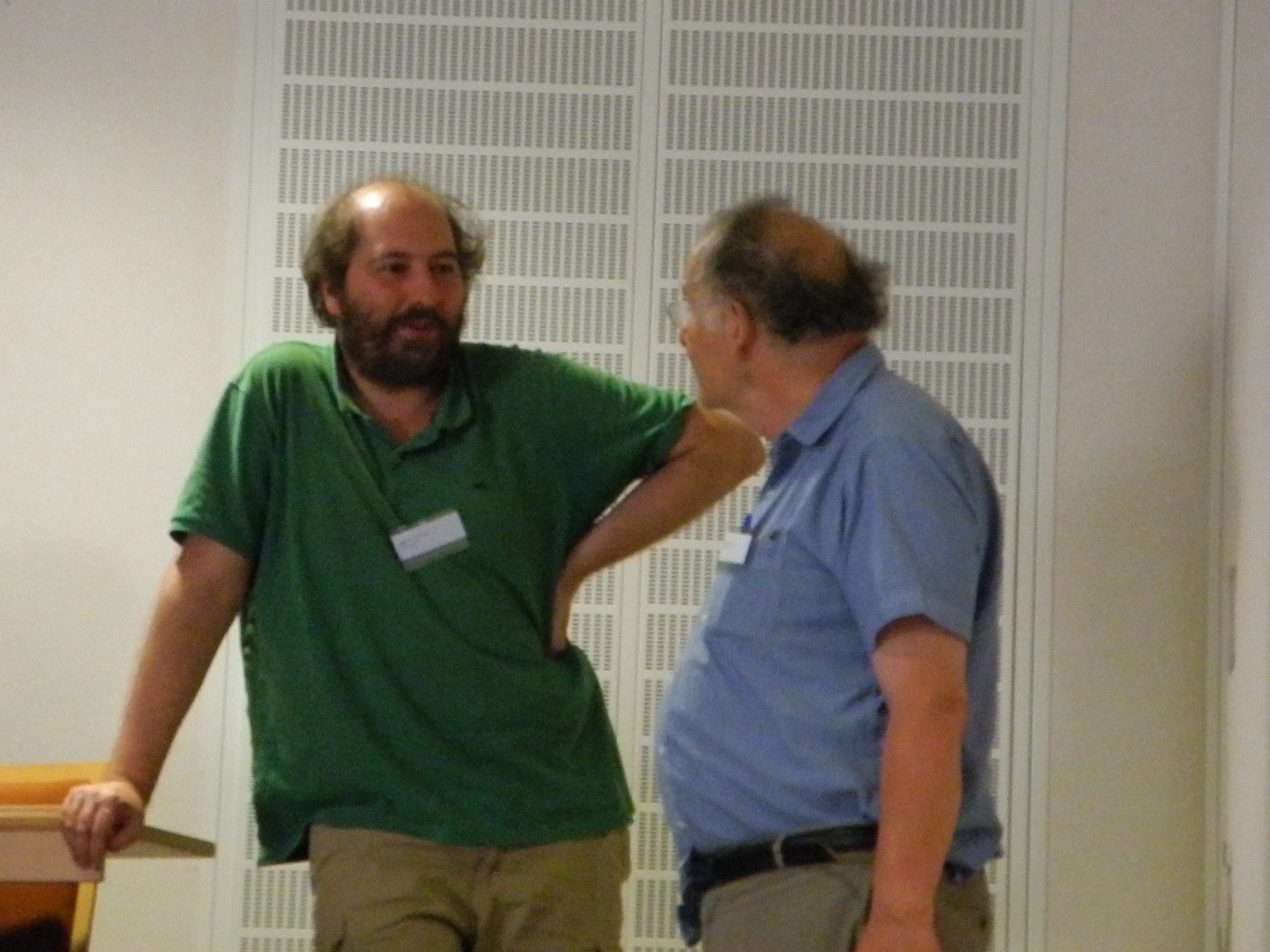
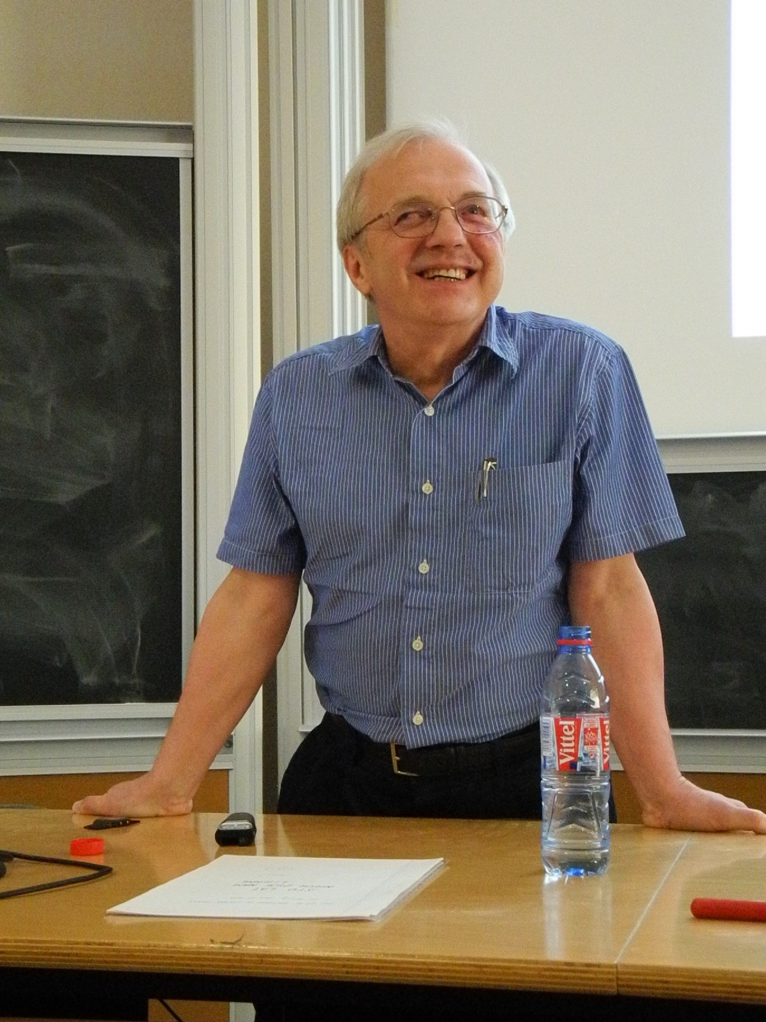
Tim Browning remembers his first meeting with Fouvry…

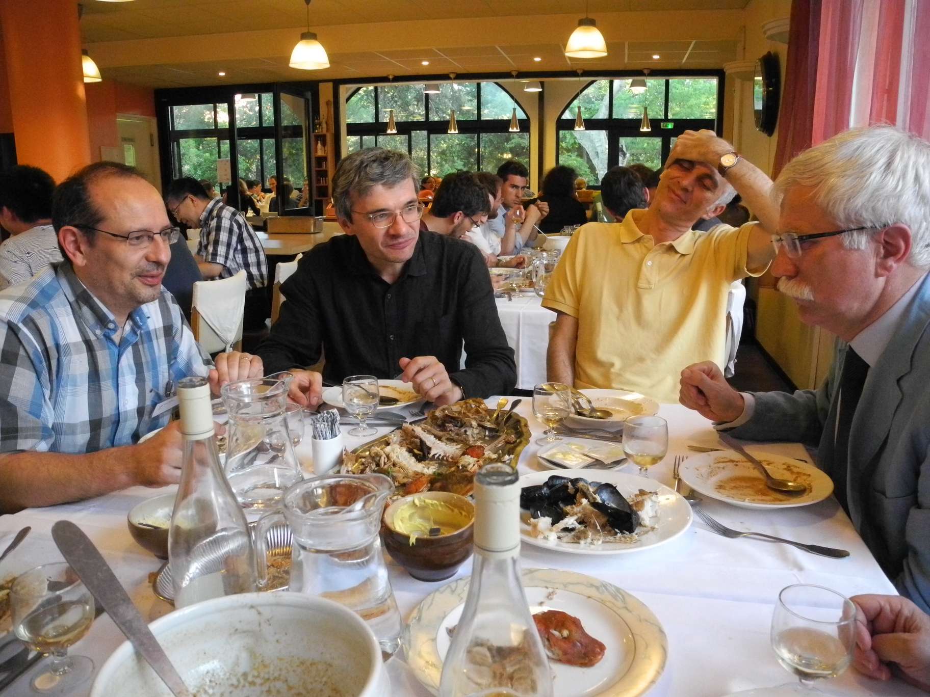
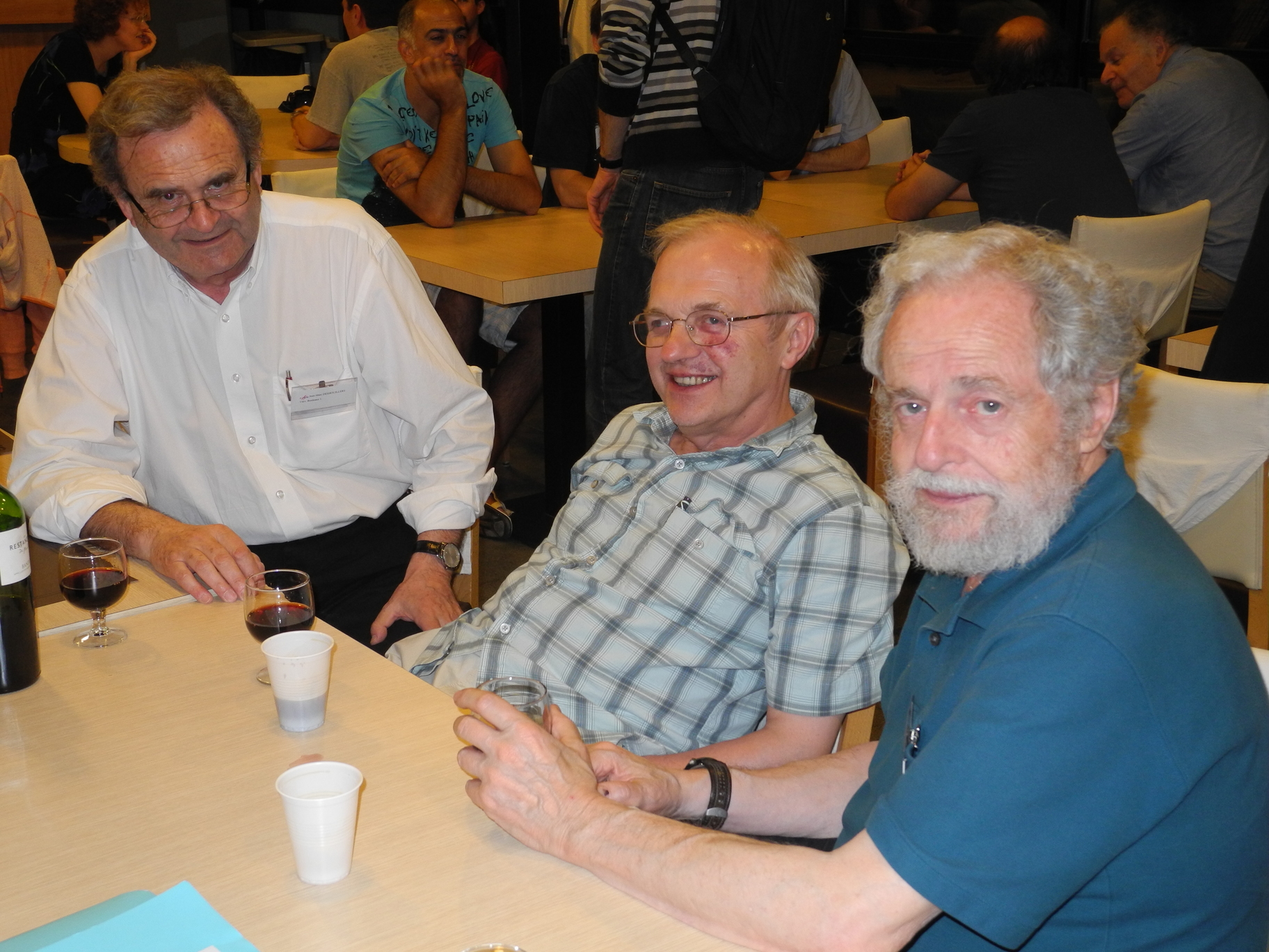
Sitting, from left to right, Philippe Michel, Régis (du Moulin) de la Bretèche, Joël Rivat (co-organizers of the meeting) and Étienne Fouvry; on the table, the Bouillabaisse: Congre, Rascasse, Saint Pierre, j’en passe, et des meilleurs.

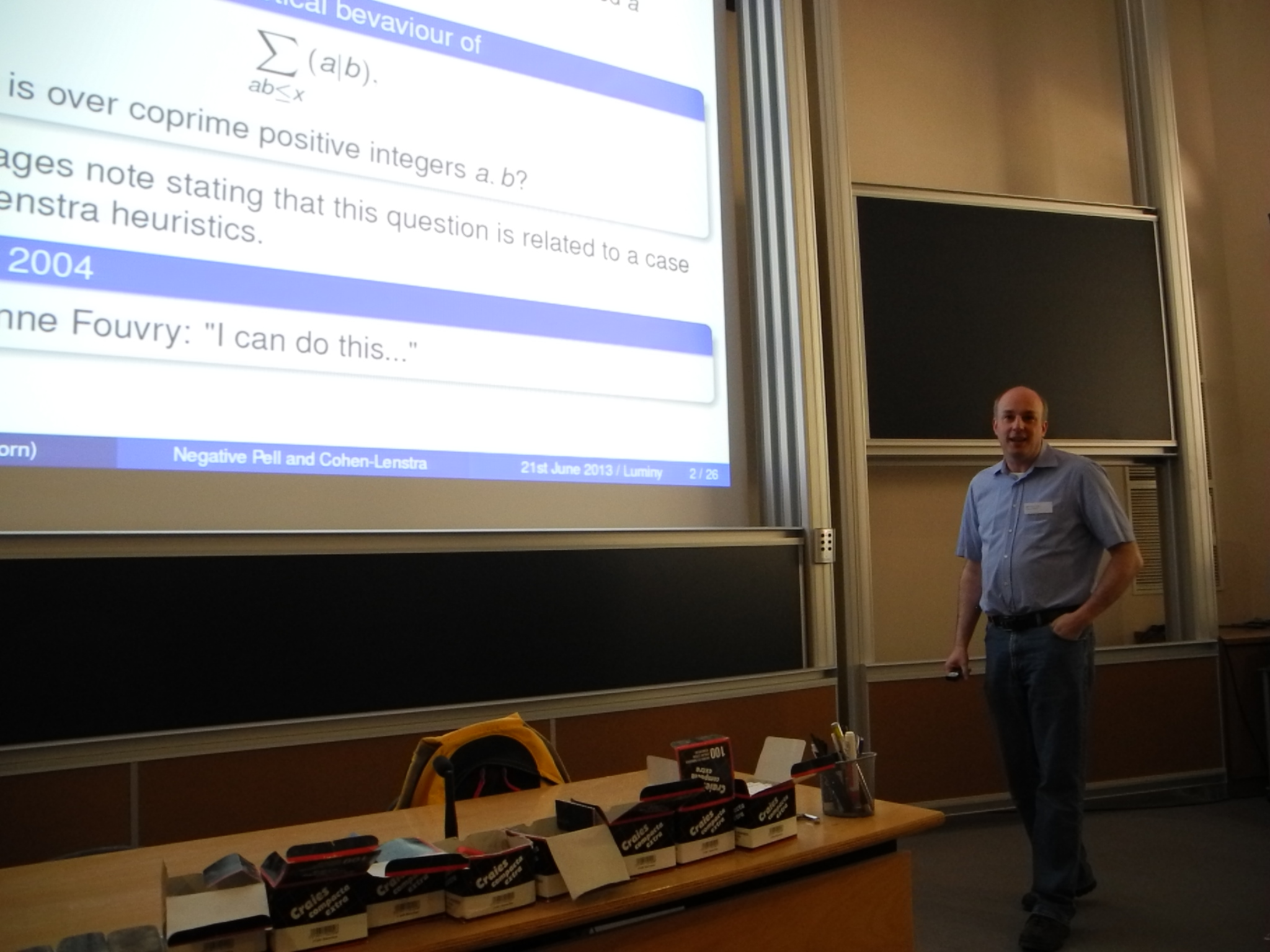
J. Klüners discussed his work with Fouvry on Cohen-Lenstra heuristics and the negative Pell equation; note the last line of the slide: “I can do this”; when collaborating with Fouvry, you have a good chance of receiving such a reassuring message at a tricky point of the work…

Here is a sketch of the argument mentioned in the previous post (which arose from the discussions with Étienne Fouvry, Philippe Michel, Paul Nelson, etc, but presentation mistakes are fully mine…).

Theorem. We have
$latex \frac{1}{Q}\sum_{r\sim R}\sum_{s\sim S}\sum_{a\bmod q,\ P(a)= 0\bmod q}\Bigl|S(a,q)-MT_q\Bigr|=O\Bigl(\frac{X}{Q\log^A X}\Bigr)$
provided
$latex Q^{3/2}S^{1/2}<N^{1-\epsilon},\quad\quad R<S,$
where
(1) we put
$latex S(a,q)=\sum_{m\sim M}\alpha_m\sum_{mn_1n_2n_3\equiv a\bmod{q},\ n_i\sim N_i}1,$
and denote by $latex MT_q$ the expected main term;
(2) the parameters are $latex X=MN=MN_1N_2N_3$, $latex Q=RS$, the modulus is $latex q=rs$, the moduli $latex r$ and $latex s$ are coprime and squarefree, and $latex P\in \mathbf{Z}[X]$ is the usual polynomial associated to an admissible tuple.

If we take $latex R=Q^{1/2-\epsilon}$ and $latex S=Q^{1/2+\epsilon}$, we get a non-trivial result for $latex Q$ as large as $latex N^{4/7}X^{-\epsilon}$.

(In fact, the special shape of $latex P$ will play no role in this argument, and any non-constant polynomial will work just as well.)

More precisely, I will give a proof which is — except for its terseness — essentially complete for $latex r$ and $latex s$ of special type, and we anticipate only technical adjustments to cover the general case — we will write this down carefully of course.

Before starting, a natural question may come to mind: given that qui peut le plus, peut le moins, can one give an analogue result for the usual divisor function? Recall that, for the latter, the (individual) exponent of distribution has been known to be at least $latex 2/3$ for a long time (by work of Linnik and Selberg independently, both using the Weil bound for Kloosterman sums.) This exponent has not been improved, even on average over $latex q$ (although Fouvry succeeded, on average over $latex q$, in covering the range $latex X^{2/3-\epsilon}\leq q\leq X^{1-\epsilon}$) despite much effort. However, Fouvry and Iwaniec (with an Appendix by Katz to treat yet another complete exponential sum over finite fields) proved already twenty years ago that one could improve it to $latex 2/3+1/48$ if one averages for a fixed $latex r \leq X^{3/8}$ over special moduli $latex q=rs$ with $latex rs^2\leq X^{1-\epsilon}$ — this gives in particular a nice earlier illustration of the usefulness of factorable moduli for this type of questions.

---

So, to work. For fixed $latex r$ and $latex s$, we begin by applying the Poisson summation formula to the three “smooth” variables $latex n_i$ (the smoothing is hidden in the notation $latex n_i\sim N_i$); the simultaneous zero frequencies $latex (h_1,h_2,h_3)=(0,0,0)$ give the main term, as they should, and the other degenerate cases are easier to handle than the contribution of the non-zero $latex h_i,$ so the main secondary term for a given $latex q$ and $latex a $ is given by
$latex S_2=\frac{N}{q^2}\sum_m \alpha_m\sum_{1\leq |h_i|\\ H_i} K_3(a\bar{m}h_1h_2h_3;q),$
where the dual lengths are $latex H_i=Q/N_i$, so that the total number of frequencies is $latex H_1H_2H_3=Q^3/N$, and where $latex K_3$ is a normalized hyper-Kloosterman sum modulo $latex rs$:
$latex K_3(u;q)=\frac{1}{q}\sum_{xyz=u}\psi_q(x+y+z),\quad\quad \psi_q(x)=e(x/q).$

(Below I will usually not repeat the range of summations when they are unchanged from one line to the next.)

Now we sum over $latex r$ and $latex s$, move the sum over $latex m$ outside, and apply the Cauchy-Schwarz inequality to the $latex r$ sum, for a fixed $latex (s,a_s,m)$, where $latex a_s$ is $latex a$ modulo $latex s$. To prepare for this step, we use the Chinese Remainder Theorem to split the condition $latex P(a)=0\bmod rs$, and to factor the hyper-Kloosterman sum as a sum modulo $latex r$ times one modulo $latex s$.

The contribution of a fixed $latex (s,a_s,m)$ is
$latex T=\frac{1}{R}\sum_{r}\sum_{P(a_r)=0\bmod{r}}\Bigl|\sum_{h_i}K_3(a\bar{m}h_1h_2h_3;rs)\Bigr|$
and we can bound
$latex T\ll H^{1/2+\epsilon} U^{1/2},$
where
$latex U=\frac{1}{R^2}\sum_{r_1,r_2} \lambda(r_1,a_1)\lambda(r_2,a_2) \sum_{1\leq |h|\ll H} \overline{K_3(a_1\bar{s}^3\bar{m}h;r_1)}K_3(a_2\bar{s}^3\bar{m}h;r_2)\overline{K_3(a_s\bar{r}_1^3\bar{m}h;s)}K_3(a_s\bar{r}_2^3\bar{m}h;s)$
for some coefficients $latex \lambda(\cdot,\cdot)$ which are bounded.

The point of this is that we have smoothed the variable $latex h=h_1h_2h_3$ by eliminating its multiplicity, and that the range of this variable can be quite long; as long as $latex H>(R^2S)^{1/2}$, completing the sum in the Polya-Vinogradov (or Poisson) style will be useful.

Now we continue with $latex U$. It is here that it simplifies matters to have $latex R<S$ and to do as if $latex r$ and $latex s$ were primes (this is a technicality which experience shows should give no loss in the final, complete, analysis.)

So we consider the sum over $latex r_1, r_2$. The diagonal contribution where $latex r_1=r_2$ is $latex \ll H^{1+\epsilon}R^{-1+\epsilon}$.

In the non-diagonal terms, we distinguish whether $latex r_1\equiv r_2\bmod s$ or not. If not, we complete the two hyper-Kloosterman sums. This gives two complete exponential sums modulo $latex r_1, r_2$ and modulo $latex s$. The latter is the Friedlander-Iwaniec sum, in its incarnation as "Borel" correlations of hyper-Kloosterman sums (see the remark at the end of our note on these sums; this identification is already in Heath-Brown's paper, and Philippe realized recently that he had also encountered them in a paper on lower bounds for exponential sums.)

Both sums give square root cancellation (using Deligne’s work, of course) except for the $latex s$ sum if $latex r_1^3\equiv \pm r_2^3\bmod s$. But we may just push these to the second case. Thus, the contribution $latex U_0$ of these non-exceptional terms gives
$latex U_0\ll (R^2S)^{1/2+\epsilon}\Bigl(\frac{H}{R^2S}+1\Bigr)$
(counting the number of complete sums in the $latex h$-interval).

On the other hand, the exceptional $latex (r_1,r_2)$ are still controlled by the diagonal terms (because of the condition $latex R<S$; there is a minor trick involved here if the cubic roots of unity exist modulo $latex s$, but I'll gloss over that.)

Now we can gather everything, and one checks that we end up with a bound
$latex \sum_{r,s}\sum_a S_2 \ll X^{\epsilon} QM\Bigl(\frac{1}{R^{1/2}}+\frac{R^{1/4}N^{1/2}}{Q^{5/4}}\Bigr).$

We need this to be $latex \ll MNQ^{-1} (\log MN)^{-A}$ for any $latex A$, and we see that we succeed as long as
$latex Q^2R^{-1/2}<N^{1-\epsilon},\quad\quad Q^{3/2}R^{1/2}<N^{1-\epsilon},$
as stated in the theorem (the second condition is implied by the first if $latex R<S$). And as mentioned just afterwards, if we have $latex R=Q^{1/2-\epsilon}$, this gives a good distribution up to $latex X^{-\epsilon}N^{4/7}$ (note that epsilons may change from one inequality to the next.)

Remark. As the reader can see, we do not use either Weyl shifts, or cancellation in Ramanujan sums. The latter might appear in a more precise analysis, however, and give some extra gain.